Instructions for Spirals and Fractals
The mathematical background can be found, for instance, in The Algorithmic Beauty of Plants, Prusinkiewicz P. and Lindenmayer, A. or in Margherite e spirali, cavolfiori e frattali, Genzo C. and Logar A.
Software: Spirals
When you start the program, you see a window like this:
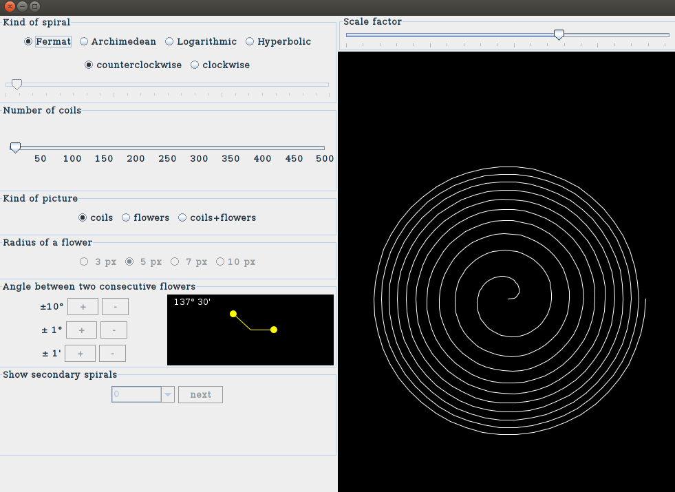
which is composed by several panels. The first panel
(Kind of spiral), allows to choose between several kind of
spirals. The most important is the Fermat spiral (in the mathematical
model we are following, it simulates
the growth of a flower calatide). You can choose the number of spiral coils
and the kind of picture (i.e. you can visualize the simple spiral, the
flowers distributed on the spiral or the spiral and the flowers on it).
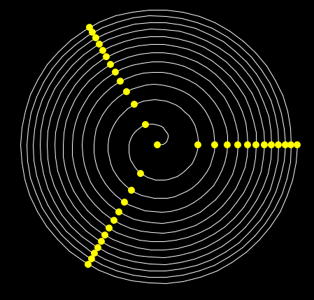
For instance here is what you get when you choose a Fermat spiral with
approximately a dozen of coils, with the button coils+flowers
selected and with the dimension of the flowers of 5 pixels:
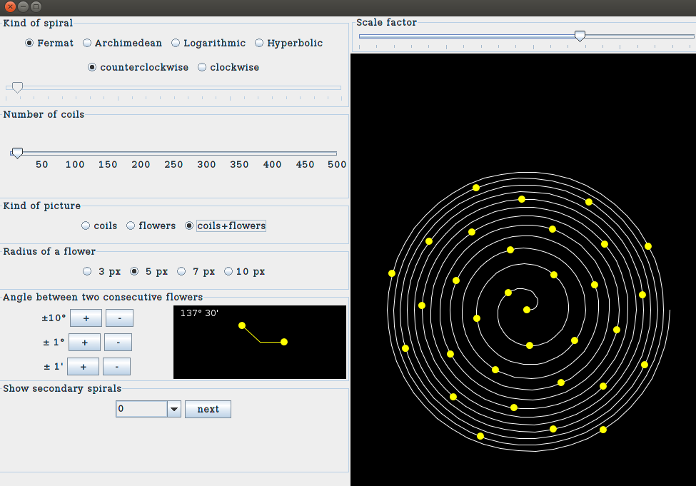
The flowers drawn on the spiral of the above picture are such that
the angle formed by two of them consecutive and the center of the spiral
is 137 degrees and 30' (the golden angle); the panel
Angle between two consecutive flowers gives some buttons to
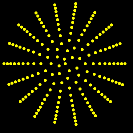
modify this angle. It is instructive to see what happens to the flowers
when we assign an angle, for instance, of 90 degrees or of 120 degrees
or 100 degrees:
we get pictures like these:
It is clear that in the first two examples the distribution of the flowers is
far from being efficient. It seems that in the third case the flowers are
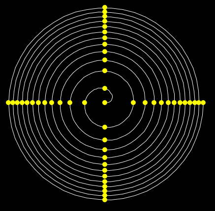
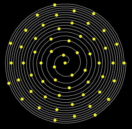
distributed with homogeneity, but if in this last case we increment the
number of coils of the spiral (for instance to 50)
(and we select the option kind of picture: flower), we get the
following distribution of the flowers:
which again shows that the flowers are not distributed in a homogeneous way.
It is interesting to experiment several values for the angle in order to
find the best value (in order to have a homogeneous distribution of the
flowers on the calatide). What happens is that the golden angle indeed seems
to be the best possible angle (the mathematical explanation require
the knowledge of the continued fractions and a property of the golden ratio,
which says that it is the most difficult number to approximate with
rationals).
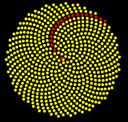
The panel show secondary spirals (active only when in the panel
kind of picture is is selected flowers or
coils+flowers) allows to visualize in red color a flower every
n on the spiral, where the number n is selected in the
text area. This panel allows to see the spiral that are usually
seen when we observe the disk flowers of a sunflower. For instance, here
is what we see in case the number of coils is approximately 250 (and
the angle between two consecutive flowers is the golden angle) and n
is 34 (a Fibonaci number). The button next visualizes other
spirals.
Software: Fractals
This software allows to obtain simple fractals.
When you start the program, you see a window like this:
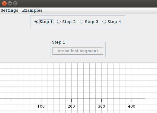
In this situation you can draw in the graph paper
some segments (using the mouse). Here is an example:
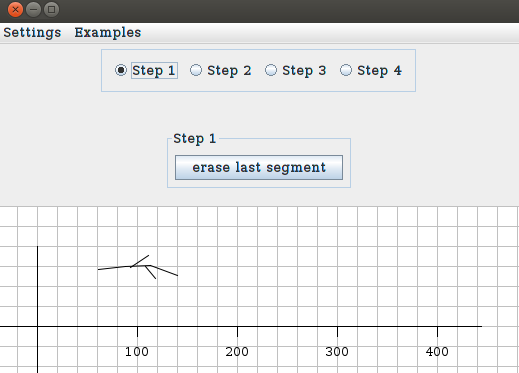
As soon as you draw the first segment, the button erase
last segment allows to erase it, (in order to allow
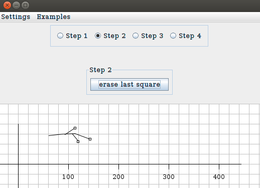
corrections). When you have completed the picture, you select
the button Step 2. Now, if you click in the graph paper,
you see that a small square appears (it can be erased with the
button erase last square). These squares represent the
points in which the branches of the fractal will start
(the number of squares you can draw is limited by 9). Here is an example
in which we put three squares on the picture drawn in Step 1:
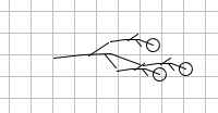
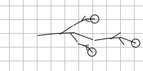
Now you select Step 3. You will see that in the
picture appears other smaller copies of the original sketch. Each of
them has a small circle. If you move the mouse on that circle, then you can
modify the scale factor and the orientation of each figure. Here is
what you get at the beginning of Step 3 and after some modification:
Note that in Step 3 you have a panel which allows to choose
between several kind of way in which you can modify the picture: rotations,
scaling, etc. By default, the button rotation and scaling is
selected. As soon as you have completed Step 3, you have given
enough information to the software in order to draw the fractal: select
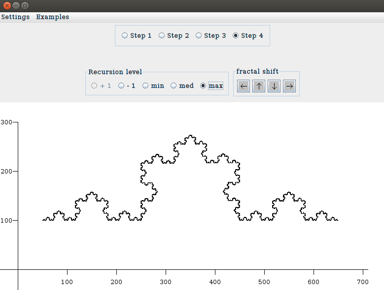
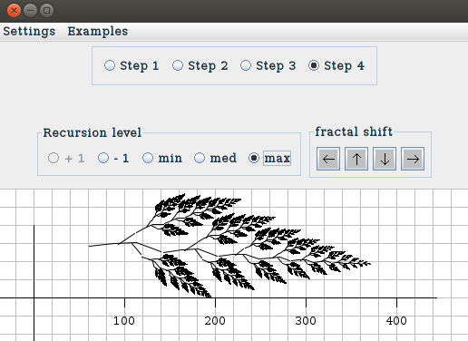
Step 4. At this point you will see the same figure you have
constructed in Step 1 but two new panels appear: Recursion
level and fractal shift. The second one allows to move the
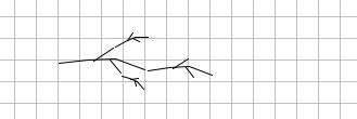
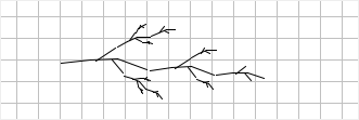
fractal, the first one has several buttons. If you press the botton
+1 several times you see the construction of the fractal.
Here is an example:
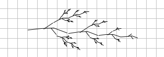
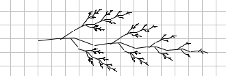
And this is the final result:
You can go back and forth between Step 4 and Step 3,
so you can slightly modify the data in Step 3 in order to
get a better result in Step 4. You can also skip from
Step 4 to Step 2 or Step 1, but in these
cases the information given in Step 3 is lost.
The menu bar has two items: Settings and Examples.
One of the items of Settings is Open I/O window.
If you select this item (in Step 3 or Step 4),
you see a new window in which you see:
- the coordinates of each segment drawn in Step 1 (they appear in the text area denoted by Segment coordinates. A sequence of 4 numbers like: 285, 80, 253, 162 represents a segment whose end points coordinates are (285, 80) and (253, 162).
- The coordinates of the branches origin;
- The angles of rotation of each branch,
- The scaling factor of each branch.
Another item in the menu Settings which probably needs an explanation is the button draw each level. If it is selected, in Step 4 you see the fractal in which all the intermediate levels are displayed, if it is not selected, you see only the last level. For instance, here is what happens when you draw the Kock snowflake in case draw each level is selected:
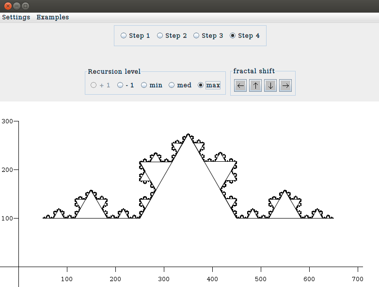
and in case when draw each level is not selected: